Active and Passive Electronic Filters: 6 + 1 application examples

24 March 2025 · Lorenzo Martini ·

HardwareAliasingAmplifiersDesignBode PlotQ FactorFiltersOTA

Active and Passive Electronic Filters: 6 + 1 application examples

Boardesign, 24/03/2025

What are filters in electronics?

Electronic filters are fundamental components in signal processing systems. Their main function is to selectively modify the frequency components of a signal, allowing some frequencies to pass while attenuating others. This characteristic makes them essential tools in numerous applications, from telecommunications to audio, from consumer electronics to industrial control systems.

Active and passive filters

Depending on how they’re built, filters can be active or passive. Active filters take on particular importance thanks to their ability to significantly improve performance compared to more traditional passive filters.

Active filters differ from passive filters because, in addition to using passive components like resistors and capacitors, they also employ active components such as op-amps or Operational Transconductance Amplifiers (OTAs). Thanks to these components, active filters offer improved performance, such as adjustable gain, high input impedance, low output impedance, and greater selectivity.

Types of Filters by Frequency Response

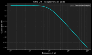
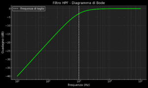
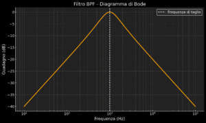
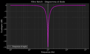
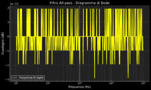
Filters are mainly distinguished by their frequency response, well represented through the Bode plot (in the figures below the signal phase isn’t shown):

Low-Pass Filter (LPF): Allows frequencies below a cutoff frequency (fc) to pass, attenuating higher-frequency components. They’re used to eliminate high-frequency noise or to extract the DC component of a signal.

High-Pass Filter (HPF): Complementary to low-pass, allowing frequencies above the cutoff to pass while attenuating lower ones. They’re used to eliminate DC offset or drift.

Band-Pass Filter (BPF): Allows only frequencies within a specific range to pass, attenuating both lower and higher frequencies. They’re fundamental in radio receivers for selecting a specific channel.

Band-stop (Notch) Filter: Attenuates frequencies in a specific range while letting both lower and higher frequencies pass. They’re used to eliminate interference at known frequencies, such as 50/60 Hz mains noise. Notch filter: A variant of the band-stop filter with an extremely narrow rejection band. Ideal for eliminating precise interference, like the 50 or 60 Hz typical of electrical mains.

All-pass filter: Doesn’t modify the amplitude of frequencies but alters the phase relationship between them. Useful in applications where correcting phase distortions is essential.

Filter Order: A Question of Poles and Zeros

The order of a filter is a parameter associated with the “steepness” of the transition between the pass band and the attenuated band. Mathematically, the order corresponds to the degree of the polynomial that describes the filter’s transfer function and is specifically tied to the number of poles and zeros in the polynomial. The higher the order, the greater the number of poles and the steeper the transition between the pass band (frequencies let through) and the stop band (frequencies attenuated). In some cases, there can also be zeros in the transfer function, which represent frequencies where the signal is completely nulled.

In summary:

Poles determine how rapidly the signal drops off in the transition zone.
Zeros define the presence of points where the signal is completely eliminated or strongly attenuated.

A first-order filter has an attenuation of 20 dB per decade (or 6 dB per octave) in the transition band. Each additional order increases this attenuation by another 20 dB per decade. For example, a second-order filter will have an attenuation of 40 dB per decade (12 dB per octave).

Higher-order filters offer sharper transitions between the pass band and the stop band, but they come with greater circuit complexity and can introduce more significant phase distortions. Choosing the filter order is therefore a trade-off between performance and implementation complexity.

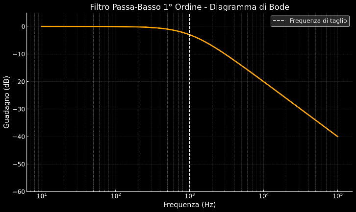
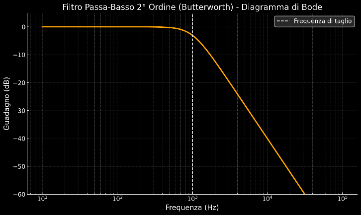
** Difference in attenuation between a first-order LPF (left) and a second-order LPF (right)**

A Mysterious Parameter: Q

The Q factor of a filter defines the selectivity and the width of the band around the filter’s center frequency. It’s essentially a quality factor: a high Q value indicates a narrower pass band and greater selectivity, while a low value corresponds to a wider band and lower selectivity. It’s essential for determining the filter’s response, its ability to isolate specific frequencies, and to manage any unwanted resonances. Mathematically, the quality factor (Q) of a filter is defined as the ratio between the center frequency (f0) and the width of the pass band (Δf), that is:

Passive Filtering Methods

1. RC Filter

The RC low-pass filter is the simplest and cheapest solution for implementing frequency filtering. It’s made up of a resistor (R) and a capacitor (C) connected in series, with the output taken across the capacitor.

How it works: At low frequencies, the capacitor behaves like an open circuit, allowing the signal to pass. As frequency increases, the capacitor’s impedance drops, progressively short-circuiting the signal to ground.

Advantages:

Simple construction and low cost
No external power supply required (passive)
High reliability
Compact size

Disadvantages:

Only first-order filter (20 dB/decade)
Cutoff frequency depends on the load
Output impedance not constant
Some attenuation even in the pass band

Practical application: In audio circuits, to eliminate high-frequency noise before analog-to-digital conversion. For example, on the microphone inputs of digital recorders, an RC filter with a cutoff frequency around 20 kHz eliminates ultrasonic interference while preserving the entire audible audio spectrum.

2. LC Band-Pass Filter

LC filters exploit the combination of inductors (L) and capacitors (C) to create resonant circuits that select specific frequency bands.

How it works: An LC circuit has a resonance at the frequency determined by f = 1/(2π√(LC)). At this frequency, the impedances of the inductor and capacitor cancel each other out, allowing the signal to pass with minimal attenuation.

Advantages:

Ability to build second-order and higher filters
Better selectivity than RC filters
Low losses in the pass band
Ability to handle high power levels

Disadvantages:

Larger size than RC filters
Sensitivity to external magnetic fields
Inductive components are more expensive and less precise
Possible presence of parasitic resonances

Practical application: In radio receivers, where LC filters are used as the “frontend” to select the desired frequency band. For example, in an AM receiver, an LC filter tuned to the frequency of the desired station (e.g., 1 MHz) separates the signal of interest from other adjacent broadcasts.

3. Crystal Filters

Crystal filters are a more sophisticated passive solution, based on the piezoelectric properties of quartz crystals or special ceramics.

How it works: They exploit the mechanical resonance phenomenon of crystals, which manifests electrically as a very-high-Q resonant circuit. This makes it possible to obtain extremely narrow, steep pass bands.

Advantages:

Extremely high selectivity (Q factor up to 100,000)
Excellent frequency stability with temperature variation
Excellent repeatability of characteristics
Compact size compared to equivalent LC filters

Disadvantages:

High cost for custom designs
Limited power-handling capability
Relatively fixed pass band (hard to tune)
Limited frequency range (typically kHz-MHz)

Practical application: In digital communication systems, like modems and GPS receivers, where high selectivity is needed to separate adjacent channels. For example, in professional satellite communication receivers, crystal filters with a bandwidth of a few kHz allow precise isolation of communication channels even in the presence of strong nearby interference.

Active Filtering Methods

4. Op-Amp Based Active Filters

Active filters combine passive components (resistors and capacitors) with op-amps, making it possible to overcome many of the limitations of purely passive filters.

How it works: Op-amps provide gain and isolation between stages, allowing multiple filter sections to be cascaded without reciprocal loading effects. The most common topologies include Sallen-Key, Multiple Feedback, and State Variable.

Advantages:

Easy to implement higher-order filters
No inductive components (problematic in terms of cost and size)
High input impedance and low output impedance
Ability to integrate gain and filtering functions

Disadvantages:

Requires external power supply
Frequency limitations due to op-amp bandwidth
Sensitivity to noise introduced by the amplifiers
Potential distortion for large-amplitude signals

Practical application: In industrial data acquisition systems, where anti-aliasing filters are crucial before analog-to-digital conversion. For example, in a vibration monitoring system, a 4th-order Butterworth active filter with a 1 kHz cutoff ensures that high-frequency signals don’t cause sampling errors, while maintaining a linear phase response in the band of interest.

5. gm-C Active Filters (Transconductance-C)

gm-C filters combine capacitors with Operational Transconductance Amplifiers (OTAs) to create filtering circuits particularly suited for high-frequency applications and integration in ICs.

How it works: OTAs convert the input voltage into a proportional current (transconductance). This driven current charges and discharges the capacitors, creating a frequency response that can be electronically tuned by modifying the transconductance of the OTAs themselves. This allows easy variation of the cutoff frequency simply by modifying a bias current or control voltage.

Advantages:

Ability to operate at high frequencies (MHz and GHz)
Precise electronic control of the cutoff frequency
High integrability in CMOS and BiCMOS technology
Complete absence of inductive components
High input impedance and good load driving capability

Disadvantages:

Sensitivity to the nonlinearities and parametric variations of the OTAs
Design complexity, especially in handling non-idealities
Possible stability problems and unwanted oscillations if not properly designed
Greater sensitivity to noise compared to other active solutions

Practical application: gm-C filters are particularly used in wireless communication systems, such as RF receivers and programmable selective filters, where it’s essential to electronically vary the pass band and quickly adapt to different communication standards. A concrete example is a software-defined radio (SDR) receiver, where a gm-C filter allows precise and rapid selection of the operating channel, maintaining low signal losses and high selectivity.

6. Wave Active Filters (WAF)

Wave Active Filters simulate traditional passive LC (ladder) filters using a network of active components like op-amps, resistors, and capacitors. They’re particularly suited to applications that require high precision and stability over time.

How it works: WAFs emulate the behavior of LC filters using op-amps configured to simulate the transfer functions typical of passive LC networks. Each active stage is designed to replicate specific frequency responses, making it easy to obtain complex, high-order filters with stable, precise performance.

Advantages:

Stability and precision of the frequency response, less influenced by thermal variations and component tolerances
Low sensitivity to parametric variations
Excellent linearity and low noise
Easy implementation of complex high-order filters without inductive components

Disadvantages:

High circuit complexity requiring more accurate design
Need for a considerable number of active and passive components
Larger footprint and higher cost compared to other types of active filters
Potential stability problems if the active network isn’t properly compensated

Practical application: WAFs find wide use in data acquisition systems and precision instrumentation, such as spectrum analyzers, high-resolution measurement instruments, and biomedical equipment. For example, in a data acquisition system for laboratory testing, a high-order Wave Active filter ensures that the acquired signal is free of interference and environmental noise, maintaining high stability over time and enabling reliable, repeatable measurements.

A Different Path: Digital Filters

Digital filters represent the most advanced and flexible filtering approach, implementing mathematical algorithms on data already converted into digital format. They’re implemented on microcontrollers, microprocessors, DSPs (Digital Signal Processors), and FPGAs (Field Programmable Gate Arrays) that have enough computational power to run them.

How it works: They process sequences of numerical samples by applying mathematical operations (multiplications and additions) according to predetermined coefficients. They’re mainly divided into finite impulse response (FIR) and infinite impulse response (IIR) filters.

Advantages:

Extreme flexibility and reconfigurability via software
Excellent precision and repeatability
Ability to implement complex transfer functions
Guaranteed stability (in FIR filters)
No component drift over time

Disadvantages:

Need for analog-to-digital conversion
Processing latency
Bandwidth limitations due to sampling frequency
Potentially high computational requirements
Possible quantization and overflow issues

Practical application: In professional audio processing, where digital filters enable extremely precise parametric equalization operations. For example, in an adaptive noise cancellation system, FIR digital filters with hundreds of coefficients make it possible to selectively identify and remove environmental noise while preserving speech quality, with applications ranging from telecommunications to voice recognition systems in noisy industrial environments.

Comparisons and Conclusions

Filtering Method**Complexity**Typical Order**Selectivity**Flexibility**Cost**Typical ApplicationsPassive RC FilterVery low1st orderLowLimitedVery lowDC decoupling, audio pre-filtersPassive LC FilterMedium2nd-4th orderMediumMediumMediumRadio receivers, audio crossoversCrystal FilterMediumHigh (Q>1000)Very highLowHighRF communications, oscillatorsActive Filter (Op-Amp)Medium-high2nd-8th orderHighHighMediumInstrumentation, hi-fi audiogm-C Filters (OTA)High2nd – 6thHighHighMedium-highWireless communications, RF receiversWave Active Filters (WAF)High3rd – 10thVery HighMediumHighData acquisition, lab instrumentationDigital FilterHighVirtually unlimitedExcellentExcellentHigh (hardware) Low (software)DSP, telecommunications, multimedia

This overview of filtering techniques highlights the great diversity of approaches available to effectively tackle the increasingly sophisticated needs of modern electronic systems. From the simple and reliable passive RC filters, ideal for basic, low-cost applications, to the complex digital filters capable of offering absolute precision and maximum operational flexibility, each method has unique characteristics that make it more or less suitable for specific application scenarios.

Passive filters, like RC, LC, and crystal filters, offer simplicity without the need for external power, making them ideal for electronic circuits that require compactness and low cost and where very high performance isn’t needed. However, the size of inductive elements, thermal and time-based drift, and performance limitations make them less flexible than active solutions.

Active filters, including those based on op-amps (Sallen-Key, Multiple Feedback), OTAs (gm-C), and Wave Active Filters (WAFs), overcome many of the limitations of passive solutions. They offer greater versatility, the ability to easily configure high-order filters, and more accurate performance control through electronic adjustments. These filters are essential in instrumentation, data acquisition, and precision audio and RF applications.

Finally, digital filters represent the ultimate expression of flexibility, reconfigurability, and precision, allowing virtually unlimited implementations in terms of order, response, and real-time adaptation to operating conditions. Nevertheless, they require analog-to-digital conversion and computational power, which makes them ideal mainly for advanced, high-performance systems.

The choice of filtering technique therefore depends on a careful analysis of technical, economic, and application requirements. A thorough understanding of the peculiarities of each type of filter enables the design of optimized electronic systems, capable of delivering excellent performance and reliability over time.

BOARDESIGN is ready to support every client in selecting, designing, and simulating the filters most appropriate to the specific needs of their projects.

Active and Passive Electronic Filters: 6 + 1 application examples